Vihar Kurama, a member of the Python Software Foundation, briefly introduced mathematics behind deep learning algorithms.
Deep Learning is a subfield of machine learning. The linear algebra is mathematical about continuous values. Many computer scientists are inexperienced in this area (traditionally computer science is more focused on discrete mathematics). To understand and use many machine learning algorithms, especially deep learning algorithms, a good understanding of linear algebra is indispensable.

Why learn mathematics?
Linear algebra, probability theory, and calculus are "languages" that express machine learning. Learning these topics helps form a deeper understanding of the underlying mechanisms of machine learning algorithms and also helps in the development of new algorithms.
If we look at a scale that is small enough, everything behind deep learning is mathematics. Therefore, it is necessary to understand the basic linear algebra before starting deep learning.
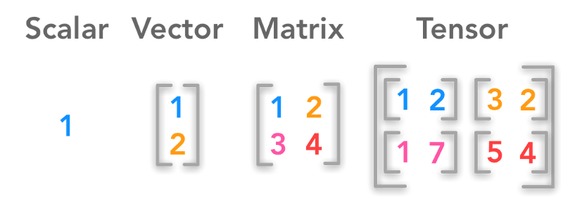
Scalar, vector, matrix, tensor; Image credit: hadrienj.github.io
The core data structures behind deep learning are scalars, vectors, matrices, and tensors. Let's programmatically use these data structures to solve the basic linear algebra problem.
Scalar
A scalar is a single number, or 0th-order tensor. x ∈ R means that x is a scalar that belongs to a set R of real numbers.
In deep learning, there are different sets of numbers. N represents a positive integer set (1,2,3,...). Z represents a set of integers, including positive, negative, and zero. Q represents a rational number set (a number that can be expressed as a ratio of two integers).
There are several built-in scalar types in Python: int, float, complex, bytes, and Unicode. Numpy has added more than twenty new scalar types.
Import numpy as np
np.ScalarType
return:
(int,
Float,
Complex,
Int,
Bool,
Bytes,
Str,
Memoryview,
Numpy.bool_,
Numpy.int8,
Numpy.uint8,
Numpy.int16,
Numpy.uint16,
Numpy.int32,
Numpy.uint32,
Numpy.int64,
Numpy.uint64,
Numpy.int64,
Numpy.uint64,
Numpy.float16,
Numpy.float32,
Numpy.float64,
Numpy.float128,
Numpy.complex64,
Numpy.complex128,
Numpy.complex256,
Numpy.object_,
Numpy.bytes_,
Numpy.str_,
Numpy.void,
Numpy.datetime64,
Numpy.timedelta64)
Among them, the data type at the end of the underscore (_) and the corresponding Python built-in type are basically equivalent.
Defining scalars and some operations in Python
The following code demonstrates some tensor arithmetic operations.
a = 5
b = 7.5
Print(type(a))
Print(type(b))
Print(a + b)
Print(a - b)
Print(a * b)
Print(a / b)
Output:
12.5
-2.5
37.5
0.6666666666666666
The following code snippet checks if the given variable is a scalar:
Import numpy as np
Def isscalar(num):
If isinstance(num, generic):
returnTrue
Else:
returnFalse
Print(np.isscalar(3.1))
Print(np.isscalar([3.1]))
Print(np.isscalar(False))
Output:
True
False
True
vector
Vectors are ordered arrays of single numbers, or, first-order tensors. Vectors are part of the vector space object. A vector space is the entire set of all possible vectors of a particular length (also called a dimension). The three-dimensional real vector space (R3) is often used to represent a three-dimensional space in the real world.

To indicate the components of the vector, the i-th scalar element of the vector is denoted as x[i].
In deep learning, vectors are often used to represent feature vectors.
Defining Vectors and Some Operations in Python
Declaration vector:
x = [1, 2, 3]
y = [4, 5, 6]
Print(type(x))
Output:
+ does not represent the addition of vectors, but the list of connections:
Print(x + y)
Output:
[1, 2, 3, 4, 5, 6]
Need to use Numpy for vector addition:
z = np.add(x, y)
Print(z)
Print(type(z))
Output:
[579]
Vector cross product
The cross product vector of two vectors, the size of which is equal to the area of ​​the parallelogram in which the two vectors are adjacent, and the direction is perpendicular to the plane where these two vectors lie:
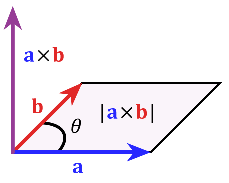
Image source: Wikipedia
Np.cross(x, y)
return:
[-36 -3]
Dot product of vector
The dot product of a vector is a scalar. For two vectors of a given length but different directions, the greater the difference in direction, the smaller the dot product.
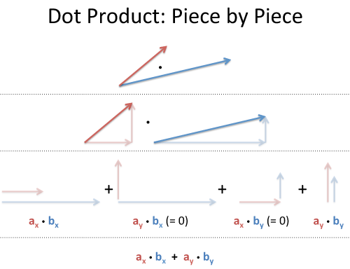
Image credit: betterexplained.com
Np.dot(x, y)
return:
32
matrix
A matrix is ​​a rectangular array of numbers, or two-order tensors. If m and n are positive integers, that is, m, n ∈ N, then an mxn matrix contains m * n numbers, m rows and n columns.
Mxn can be expressed in the following form:
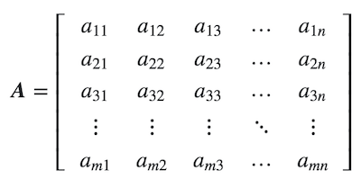
Sometimes abbreviated as:

Defining matrices and some operations in Python
In Python, we use the numpy library to create an n-dimensional array, which is a matrix. We pass the list to the matrix method to define the matrix.
x = np.matrix([[1,2],[3,4]])
x
return:
Matrix([[1, 2],
[3, 4]])
The element mean of the 0th axis of the matrix:
X.mean(0)
return:
Matrix([[2., 3.]]) # (1+3)/2, (3+4)/2
The elemental mean of the 1st axis of the matrix:
X.mean(1)
return:
z = x.mean(1)
z
return:
Matrix([[1.5], # (1+2)/2
[3.5]]) # (3+4)/2
The shape attribute returns the shape of the matrix:
Z.shape
return:
(twenty one)
Therefore, the matrix z has 2 rows and 1 column.
By the way, the shape property of the vector returns a tuple consisting of a single number (the length of the vector):
Np.shape([1, 2, 3])
return:
(3,)
The scalar shape property returns an empty ancestor:
Np.shape(1)
return:
()
Matrix Addition and Multiplication
The matrix can be added and multiplied with scalars and other matrices. These operations are mathematically well-defined. Machine learning and deep learning often use these operations, so it is necessary to become familiar with these operations.
Sum the matrix:
x = np.matrix([[1, 2], [4, 3]])
X.sum()
return:
10
Matrix-scalar addition
Add a given scalar to each element of the matrix:
x = np.matrix([[1, 2], [4, 3]])
x + 1
return:
Matrix([[2, 3],
[5, 4]])
Matrix-scalar multiplication
Similarly, matrix-scalar multiplication is to multiply each element of the matrix by a given scalar:
x * 3
return:
Matrix([[ 3, 6],
[12, 9]])
Matrix-Matrix Addition
The same shape of the matrix can be added. The sum of the elements of the corresponding positions of the two matrices is taken as the element of the new matrix, and the shape of the new matrix is ​​the same as the original two matrices.
x = np.matrix([[1, 2], [4, 3]])
y = np.matrix([[3, 4], [3, 10]])
The x and y shapes are (2, 2).
x + y
return:
Matrix([[ 4, 6],
[ 7, 13]])
Matrix-Matrix Multiplication
A matrix of shape mxn is multiplied with a matrix of shape nxp to obtain a matrix of shape mxp.
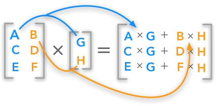
Image Source:hadrienj.github.io
From a programming point of view, an intuitive explanation of matrix multiplication is that one matrix is ​​data and the other matrix is ​​a function (operation) that will be applied to the data:
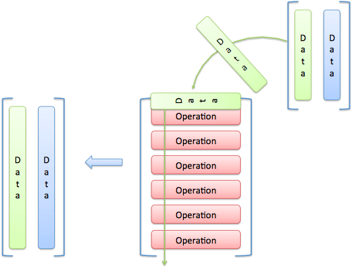
Image credit: betterexplained.com
x = np.matrix([[1, 2], [3, 4], [5, 6]])
y = np.matrix([[7], [13]]
x * y
return:
Matrix([[ 33 ],
[73],
[113]])
In the above code, the shape of matrix x is (3, 2) and the shape of matrix y is (2, 1), so the shape of the resulting matrix is ​​(3, 1). If the number of columns of x is not equal to the number of rows of y, then x and y cannot be multiplied. Forcing the multiplication will cause the shapes not aligned.
Matrix transpose
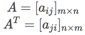
The matrix transposes the rows and columns of the original matrix (rows become columns, columns become rows), ie:
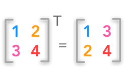
x = np.matrix([[1, 2], [3, 4], [5, 6]])
x
return:
Matrix([[1, 2],
[3, 4],
[5, 6]])
Transpose the matrix using the transpose() method provided by numpy:
X.transpose()
return:
Matrix([[1, 3, 5],
[2, 4, 6]])
Tensor
More general than scalars, vectors, and matrices are tensor concepts. In physical science and machine learning, it is sometimes necessary to use tensors over second order (remember? scalars, vectors, and matrices can be regarded as 0, 1, 2 order tensors, respectively).
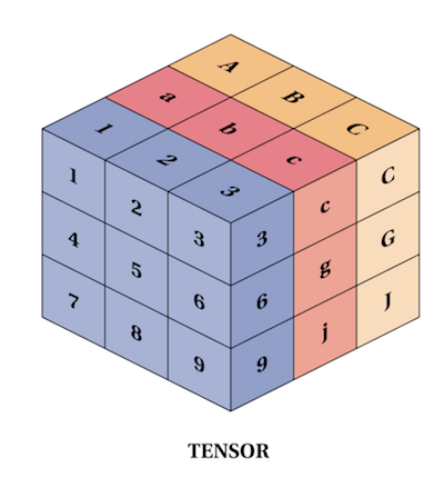
Image Source:refactored.ai
Define tensors and some operations in Python
The tensor can of course also be represented by numpy (a tensor that exceeds second-order is nothing but a two-dimensional array):
Import numpy as np
t = np.array([
[[1,2,3], [4,5,6], [7,8,9]],
[[11,12,13], [14,15,16], [17,18,19]],
[[21,22,23], [24,25,26], [27,28,29]],
])
T.shape
return:
(3, 3, 3)
Tensor addition
s = np.array([
[[1,2,3], [4,5,6], [7,8,9]],
[[10, 11, 12], [13, 14, 15], [16, 17, 18]],
[[19, 20, 21], [22, 23, 24], [25, 26, 27]],
])
s + t
return:
Array([[[ 2, 4, 6],
[ 8, 10, 12],
[14, 16, 18]],
[[21, 23, 25],
[27, 29, 31],
[33, 35, 37]],
[[40, 42, 44],
[46, 48, 50],
[52, 54, 56]]])
Tensor multiplication
What s * t gets is Hadamard Product (element-wise multiplication). It multiplies each element of the tensor s and t. The resulting product is the corresponding position of the result tensor. element.
s * t
return:
Array([[[ 1, 4, 9],
[ 16, 25, 36],
[ 49, 64, 81]],
[[110, 132, 156],
[182, 210, 240],
[272, 306, 342]],
[[399, 440, 483],
[528, 575, 624],
[675, 728, 783]]])
The Tensor Product needs to be calculated using numpy's tensordot method.

Image source: Wikipedia
Calculate s ⊗ t:
s = np.array([[[1, 2], [3, 4]]])
t = np.array([[[5, 6], [7, 8]]])
Np.tensordot(s, t, 0)
return:
Array([[[[[[ 5, 6],
[ 7, 8]]],
[[[10, 12],
[14, 16]]]],
[[[[15, 18],
[21, 24]]],
[[[20, 24],
[28, 32]]]]]])
Among them, the last parameter 0 represents the tensor product. When this parameter is 1, it represents a tensor dot product. This operation can be regarded as a generalization of the vector dot product concept. When this parameter is 2, it represents a tensor double. Contraction) This operation can be viewed as a generalization of the concept of matrix multiplication.
Of course, since tensors are commonly used for deep learning, we often use the deep learning framework directly to express tensors. For example, in PyTorch, create a tensor of shape (5, 5) and fill it with a floating point number:
Torch.ones(5, 5)
return:
Tensor([[ 1., 1., 1., 1., 1.],
[ 1., 1., 1., 1., 1.],
[ 1., 1., 1., 1., 1.],
[ 1., 1., 1., 1., 1.],
[ 1., 1., 1., 1., 1.]])
Regular GFCI Receptacle Outlet
Lishui Trimone Electrical Technology Co., Ltd , https://www.3gracegfci.com