Averaging is one of the most common methods of reducing the inherent uncertainty of a measurement system. Performing multiple measurements and averaging the results can reduce the impact of measurement randomness. Most of today's measuring instruments have an average function. Instruments usually do not directly output noise-containing results. Instead, they measure hundreds of times, calculate the average value, and output the average value as a result. However, as described below, the average power in the spectrum analyzer sometimes leads to incorrect results.
The experiments in this paper will refer to the power measurements of spectrum analyzers from two different vendors. However, the conclusions of this paper apply to any spectrum analyzer that uses the “post-processing average methodâ€.
The first misconception: Average the rms power to get the average power of a trajectory with zero span (or a portion thereof). In order to better refute this point of view, it is necessary to first understand the average mathematical definition. As shown in Equation 1: MAVE is the average of N measurements of a test, where Mi is the result of each measurement.
In this example, the results of Instrument A and Instrument B are within acceptable limits (eg ±1 dB) and all tests are tested with a frequency span of zero ZS (zero span). The time spectrum analyzer measures the relationship of the power of this frequency over time at a fixed frequency. This is not a deliberate choice of ZS mode, in fact, the average problem also exists in the traditional frequency domain scanning test.

In both cases, the ZS mode is used to measure the zero channel power ratio ACPR (adjacent-channel-power-raTIo). For modern spectrum analyzers that use digital IF filters, this measurement capability is necessary to measure power multiple times at frequencies that deviate from the center of the carrier at different frequency offsets without retuning the center frequency of the spectrum analyzer. .
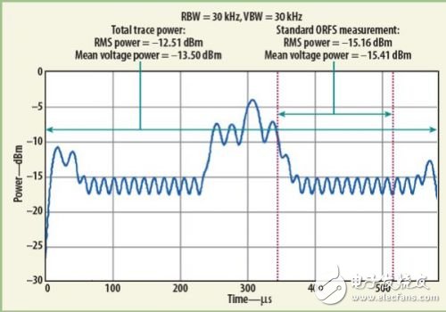
Figure 1 shows a GSM time slot pulse signal in ZS mode. The blue curve is the power envelope of the pulse. What is measured here is the "RF output modulation spectrum", also known as ACPR measurement.

A lot of results can be obtained from this curve, such as maximum peak power, minimum power and average power. Finding the maximum/minimum power is conceptually very intuitive, and the instrument can directly search for the maximum/minimum point from the trajectory.
The easiest way to calculate the average power (and of course correct) is to average the measurement points within the red limit. As shown in Equation 2, where N is the number of points within the red limit, the Pith point is the power of the ith point.

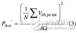
The problem is that instrument manufacturers are inconsistent with the method of power averaging. One of the manufacturers is calculated according to Equation 2; however, another manufacturer converts the power into a voltage, averages the voltage, and converts the average voltage into an average power, as shown in Equation 3.

Since the difference between the average values ​​of the two instruments is small, it is difficult to see that one of the instruments uses Equation 2, and the other uses Equation 3. It is necessary to take multiple sets of trajectories from the two instruments and average them until the match is found. In the example of Figure 1, the difference between the instrument using the "true rms" average power algorithm (hereafter referred to as RMS power) and the instrument using "voltage average" power is 0.25 dB (the former is 0.25 higher than the latter). dB). This difference may be simply thought of as an individual difference between instruments. Although 0.25dB looks small, when the required accuracy is only ±1dB, 0.25dB is a bit large. If the average power of the entire pulse is measured (the modulation spectrum measures the power from 50% to 90% of the pulse), the difference will increase to about 1 dB. This value will be close to the tolerance of the error between the instruments we require.
The "voltage average" power represents the "mean-squared" power (as in Equation 3), while the "mean square power" is the "mean-square" power. From the knowledge of statistics we can conclude that the difference between the two is the amplitude change. That is to say, the difference between the output power of the two instruments is the amplitude change. Moreover, the "mean square power" is always greater than the "RMS power" average voltage power.
The second misconception about power averaging is that averaging power is always done in linear units (watts). In fact, many instruments often use logarithmic averaging. Also using the above example, assuming that the noise in the test has a great influence, in order to remove the noise, it is decided to measure multiple sets of trajectories and average the trajectories. The GSM standard specifies that the measurement of the ORFS modulation spectrum requires averaging of 200 pulses. Equation 4 is the corresponding calculation formula, where PTrace i is the average of a single trajectory calculated using Equation 2 or Equation 3.

Of course, it is reasonable to average the linear expression of this power (in watts), but many instruments provide logarithmic averaging. In this example, the power in dBm is averaged. For example, find the average of 1 and 3 dBm: If the linear average result is: (1.25 mW 2mW) / 2 = 1.62 mW = 2.11 dBm; but the result of logarithmic averaging is: (1 dBm 3 dBm) / 2 = 2 dBm. Therefore, the log-averaged result introduces an error of 0.11 dB.
It should be noted that the magnitude of the error caused by the logarithmic averaging is related to whether the signal is repeated. Although the log-average method is wrong, for repeated signals, the log-average and linear-average results are consistent. It should be noted that the repeated signal referred to here refers to each cycle, and its power versus time relationship is exactly the same.
It must be borne in mind that non-repetitive signals introduce errors that, if not noticed, often result in large errors in the laboratory's measurement data and the practical environment. Because in the laboratory, we usually use a very good "arbitrary waveform generator" (ARB) as a signal source, this source is usually a repeated play of a waveform. But the signals in the practical environment are certainly not repetitive. However, as long as the power difference between different cycles is not very large, the log-average and linear average errors will not be large.
Another thing to note is the average algorithm problem of the corresponding "points and points" between each track measured each time the trajectory is averaged. Similarly, signal repeatability can affect errors caused by logarithmic averaging. Here, each point on the trajectory is averaged together with corresponding points on other trajectories, and the result is taken as the average of this point.
Similarly, each point on the trajectory is averaged along with the corresponding point on the other trajectory (the same x-axis) to yield an average trajectory. Here the x-axis corresponds to the time, of course, also applies to the frequency. As before, linear or logarithmic averaging can be used here. This way, after averaging each point on the x-axis, you get an average trajectory. If the signal is repetitive, the linear average and logarithmic average results are the same because the power at each point on the x-axis is the same on each measured trajectory.
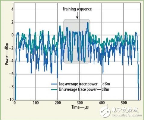
What happens when the signal under test is not repeated? Figure 2 shows the results of logarithmic and linear averaging for 20 different EDGE signals. Of course, the two curves will be different, and it can be seen that the log-average result is smaller than the linear one. Figure 3 shows the difference between each point of the two curves. Note that, as we expected, the trajectories of the training sequences are completely coincident with the training sequence (Translator's Note: the part used for synchronization and channel estimation is completely repetitive).

Conecting Terminals Without Screws
Conecting Terminals Without Screws,Cold Pressing Terminals,Low Pressure Cold Shrinkage Terminal,Cold Shrinkage Cable Terminals
Taixing Longyi Terminals Co.,Ltd. , https://www.lycopperterminals.com