Editor's note: DataScience+ author Anish Singh Walia provides an overview of commonly used neural network optimization algorithms.
Have you ever thought about what optimization algorithm should be used for your neural network model? Should we use gradient descent or stochastic gradient descent or Adam?
What is an optimization algorithm?
The optimization algorithm helps us minimize (or maximize) an objective function (another name for the error function) E(x), which is nothing but a mathematical function that depends on the internal learnable parameters of the model. The internal learnable parameters are used to Calculate the predicted target value (Y) based on a set of inputs (X). For example, the weight (W) and bias (b) of the neural network are called the internal learnable parameters of the neural network. These parameters are used to calculate the output value and learn and update in the direction of the optimization plan, that is, in the network training Minimize losses in the process.
The internal parameters of the model play an extremely important role in the effect and efficiency of the training network to produce accurate results. They affect the learning process of our model and the output of the model. This is the reason why we use a variety of optimization strategies and algorithms to update and calculate the appropriate optimal values ​​of these model parameters.
Type of optimization algorithm
Optimization algorithms can be divided into two categories:
First Order Optimization Algorithms
These algorithms minimize or maximize the loss function E(x) based on the gradient value of the loss function on the parameters. The most widely used first-order optimization algorithm is gradient descent. The first derivative tells us whether the function falls or rises at a certain point. Basically, the first derivative provides a straight line tangent to a point on the error plane.
What is the gradient of a function?
The gradient is nothing but a vector, which is a multivariate generalization of the derivative (dy/dx). The derivative (dy/dx) is the instantaneous rate of change of y relative to x. The main difference is that the gradient is used to calculate the derivative of a multivariate function, through the partial derivative calculation. Another major difference is that the gradient of the function generates a vector field.
The gradient is represented by the Jacobian matrix-a matrix containing the first partial derivative (gradient).
In simple terms, the derivative is defined on the unit function, and the gradient is defined on the multivariate function. We will not discuss more about calculus and physics.
Second Order Optimization Algorithms (Second Order Optimization Algorithms)
The second-order method uses a second-order derivative to minimize or maximize the loss function. The second-order method uses the Hessian matrix-a matrix containing second-order partial derivatives. Due to the high cost of calculating the second derivative, the second-order method is not as common as the first-order method. The second derivative tells us whether the first derivative is rising or falling, which indicates the curvature of the function. The second derivative provides a quadratic plane that fits the curvature of the error plane.
Although the calculation of the second derivative is expensive, the advantage of the second-order optimization algorithm is that it does not ignore the curvature of the error plane. In addition, in terms of performance at each step, the second-order optimization algorithm is better than the first-order optimization algorithm.
Learn more about the second-order optimization algorithm: https://web.stanford.edu/class/msande311/lecture13.pdf
Which type of optimization algorithm should be used?
Currently, the first-order optimization technique is easier to calculate, takes less time, and converges quite quickly on large data sets.
Only when the second derivative is known, the second-order technique is faster, otherwise such methods are always slower and more computationally expensive (both in time and memory).
However, sometimes Newton's second-order optimization algorithm can descent by more than one step, because the second-order technique will not fall into the slow convergence path near the saddle point, and the gradient descent will sometimes sink and fail to converge.
The best way to know which type of algorithm converges faster is to try it yourself.
Gradient descent
Gradient descent is the basic and most important technology for training and optimizing intelligent systems.
Oh, gradient descent-find the minimum, control the variance, then update the parameters of the model, and finally lead us to convergence
θ=θ−η⋅∇J(θ) is the parameter update formula, where η is the learning rate, and ∇J(θ) is the gradient of the loss function J(θ) on the parameter θ.
Gradient descent is the most popular algorithm for optimizing neural networks. It is mainly used to update the weights of neural network models, that is, to update and adjust model parameters in a certain direction in order to minimize the loss function.
We all know that training neural networks is based on a well-known technique called back propagation. In the training of the neural network, we first perform forward propagation, calculate the dot product of the input signal and the corresponding weight, and then apply the activation function. The activation function introduces nonlinearity in the process of converting the input signal to the output signal. This pair of models It is very important, so that the model can learn almost any function mapping. After that, we backpropagate the error of the network and update the weight value based on gradient descent, that is, we calculate the gradient of the error function (E) on the weight (W), which is the parameter, and then use the opposite of the gradient of the loss function The direction update parameter (here is the weight).
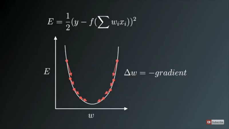
The weights are updated in the opposite direction of the gradient
In the figure above, the U-shaped curve is the gradient (slope). As you can see, if the weight (W) value is too small or too large, then we will have a large error, so we want to update and optimize the weight to be neither too small nor too large, so we follow the opposite direction of the gradient Decrease until a local minimum is found.
Gradient descent variant
The traditional gradient descent will calculate the gradient for the entire data set, but only one update, so it is very slow, and it is even more difficult for a data set that is too large to store. The size of the update is determined by the learning rate η, while ensuring that it can converge to the global minimum on the convex error plane and to the local minimum on the non-convex error plane. In addition, standard gradient descent computes redundant updates on large data sets.
The above standard gradient descent problem has been corrected in stochastic gradient descent.
1. Stochastic gradient descent
Stochastic gradient descent (SGD) updates the parameters for each training sample. Usually it is a much faster technique. It is updated one at a time.
θ=θ−η⋅∇J(θ;x(i);y(i))
Due to these frequent updates, parameter updates have high variance, which leads to severe fluctuations in the loss function. This is actually a good thing, because it helps us discover new and possibly better local minima, while the standard stochastic gradient descent only converges to the basin minima as mentioned earlier.
However, the problem with SGD is that due to frequent updates and fluctuations, it eventually complicates the convergence process, and will continue to overshoot due to frequent fluctuations.
However, if we slowly decrease the learning rate η, SGD exhibits the same convergence mode as the standard gradient descent.
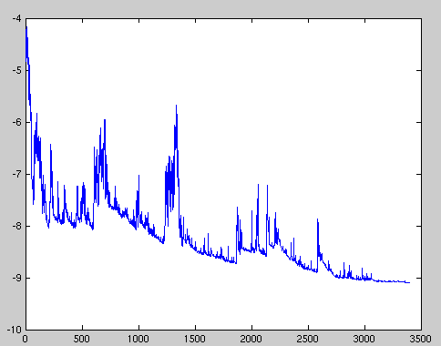
The loss function fluctuates sharply, so we may not be able to get the parameters that minimize the loss value
The high variance parameter update and unstable convergence are corrected in another variant called Mini-Batch Gradient Descent.
2. Mini-batch gradient descent
To avoid all the problems and shortcomings of SGD and standard gradient descent, you can use mini-batch gradient descent, which absorbs the advantages of both technologies and performs batch updates each time.
The advantages of using mini-batch gradient descent are:
The variance of parameter updates is reduced, leading to better and more stable convergence in the end.
The highly optimized matrix operations commonly found in the most advanced deep learning libraries can be used to calculate mini-batch gradients extremely efficiently.
The commonly used mini-batch size is 50 to 256, but it may be different depending on the application and the problem.
Small batch gradient descent is a typical choice for training neural networks today.
PS In fact, many times SGD refers to small batch gradient descent.
Challenges faced by gradient descent and its variants
Choosing the right learning rate can be difficult. A learning rate that is too small results in a slowness that makes people doubt the convergence of life. When looking for the optimal parameter value to minimize the loss, taking baby-like steps directly affects the total training time, making it too long. An excessively large learning rate may hinder convergence, causing the loss function to fluctuate around the minimum value, or even embark on a divergent path of no return.
In addition, the same learning rate is applied to all parameter updates. If our data is sparse and our features have very different frequencies, we may not want to update all features to the same degree, but want to make larger updates on features that rarely appear.
Another key challenge in minimizing the highly non-convex error function commonly seen in neural networks is to avoid falling into numerous suboptimal local minima. In fact, the difficulty lies not only in the local minimum, but also in the saddle point, that is, the point where the slope of one dimension rises and the slope of the other dimension drops. These saddle points are usually surrounded by plateaus with equal errors. As we all know, this makes it difficult for SGD to escape because the gradient is close to zero in all dimensions.
Optimize gradient descent
Now we will discuss various algorithms to further optimize gradient descent.
momentum
The high variance oscillation of SGD makes it difficult to converge, so people invented a technology called Momentum, which accelerates SGD by navigating in related directions and slowing down oscillations in unrelated directions. In other words, it adds the update vector of the previous step to the current update vector, multiplied by a coefficient γ.
V(t)=γV(t−1)+η∇J(θ)
Finally, we update the parameters by θ=θ−V(t).
The momentum term γ is usually set to 0.9, or a similar value.
The momentum here comes from the concept of momentum in classical physics. When we throw a ball down a hillside, the ball collects momentum as it rolls down the hillside, and its speed keeps increasing.
The same thing happened in our parameter update process:
It leads to faster and more stable convergence.
It reduces oscillations.
The momentum term γ expands and updates in the dimension where the gradient points in the same direction, and shrinks and updates in the dimension where the gradient direction changes. This reduces unnecessary parameter updates, leads to faster and more stable convergence, and reduces oscillations.
Nesterov accelerated gradient
Yurii Nesterov discovered a problem with momentum:
A ball that rolls down a hillside blindly with the slope is not satisfactory. We hope to have a smarter ball, have a certain idea of ​​where it is, and know that it slows down when the slope becomes upward.
In other words, when we reach the minimum value, that is, the lowest point of the curve, the momentum is quite high. Because of the high momentum, the optimization algorithm does not know where to slow down, which may cause the optimization algorithm to completely miss the minimum value and then Then move up.
Yurii Nesterov published a paper in 1983 that solved the problem of momentum. We now call the proposed strategy Nesterov Accelerated Gradient (NAG).
Nesterov proposed that we first make a big jump based on the previous momentum, then calculate the gradient, and then make corrections accordingly, and update the parameters according to the corrections. Pre-update can prevent the optimization algorithm from going too fast to miss the minimum value, making it more sensitive to changes.
NAG is a way to provide predictive capabilities for momentum items. We know that we will use the momentum term γV(t−1) when we update the parameter θ. Therefore, calculating θ−γV(t−1) can provide an approximate value of the next position of the parameter. In this way, we can "foresee the future" by calculating the gradient on the approximate value of the parameter's future position:
V(t)=γV(t−1)+η∇J( θ−γV(t−1))
Then we also update the parameters by θ=θ−V(t).
For more details about NAG, please refer to the cs231n course.
Now, we have been able to adjust the update amplitude according to the slope of the error function and accelerate the SGD process. We also hope to adjust the update amplitude according to the importance of different parameters.
Adagrad
Adagrad allows the learning rate η to be adjusted based on parameters, making larger updates for infrequent parameters and smaller updates for frequent parameters. Therefore, it is very suitable for processing sparse data.
Adagrad uses a different learning rate for each parameter θ at each time step, and the size of the learning rate is based on the past gradient of the parameter.
Before, we updated all the parameters θ at once, because each parameter θ(i) uses the same learning rate η. Since Adagrad uses a different learning rate for each parameter θ(i) at each time step t, we first calculate the update of Adagrad on each parameter, and then vectorize it. Let gi,t be the gradient of the loss function of the parameter θ(i) at time step t, then the formula of Adagrad is:
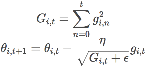
In the above formula, ϵ is a smoothing factor to avoid dividing by zero.
From the above formula, we can see:
If Gi,t in a certain direction is smaller, the corresponding learning rate is larger, that is to say, larger updates are made for the parameters that do not appear frequently.
As time goes by, Gi,t gets bigger and bigger, so the learning rate gets smaller and smaller. Therefore, we do not need to manually adjust the learning rate. In most Adagrad implementations, η uses the default value of 0.01. This is a big advantage of Adagrad.
Since Gi,t is the sum of squares, each term is positive. Therefore, as the training process progresses, Gi,t will continue to grow. This means that the learning rate will continue to decrease, the model will converge more and more slowly, training will take a long time, and even the final learning rate will be so small that the model stops learning completely. This is the main flaw of Adagrad.
Another algorithm, AdaDelta, fixes the learning rate decay problem of Adagrad.
AdaDelta
AdaDelta tries to solve Adagrad's learning rate decay problem. Unlike Adagrad accumulates all past square gradients, Adadelta limits the range of accumulation and only accumulates past gradients in a window of fixed size w. In order to improve efficiency, Adadelta does not store w square gradients, but the average of the square gradients in the past. In this way, the dynamic mean of time step t depends only on the previous mean and the current gradient.

Among them, the value of γ is similar to the momentum method, around 0.9.
Similar to Adagrad, Adadelta's formula is:

Since the denominator part fits the definition of the mean square error of the gradient:

This is actually the formula of RMSprop. RMSprop was proposed by Geoffrey Hinton and was not published in the form of a paper. See its csc321 course.
Adadelta and RMSProp were developed independently of each other at about the same time, both to solve Adagrad's learning rate decay problem.
In addition, in the standard Adadelta algorithm, symmetric with the denominator, the numerator η can also be replaced with RMS[Δθ]t-1:

This eliminates η! In other words, we do not need to specify the value of η.
The improvements we have made so far
Calculate different learning rates for each parameter.
Calculate momentum at the same time.
Prevent the learning rate from decay.
What can be improved?
Now that we have calculated the learning rate separately for each parameter, why not calculate the momentum change for each parameter separately? Based on this idea, people proposed the Adam optimization algorithm.
Adam
Adam stands for Adaptive Moment Estimation.
Straightforward, let's look directly at Adam's formula:

Is there a feeling of deja vu? You feel right, this is very similar to RMSProp or Adadelta's formula:

So, the question is, what are these vt and mt? Don't worry, we will give the definition of both immediately.
Let's take a look at vt first:

Yo! This is the past mean squared gradient in Adadelta or RMSProp! Just changed a few letters, replaced γ with β2, and replaced E[g2] with v.
Let's take a look at the definition of mt:

Huh? This seems a bit similar to the definition of momentum?
V(t)=γV(t−1)+η∇J(θ)
γ is replaced by β1, and both ∇J(θ) and gt are gradients. Of course, there is another coefficient that is different, it's just a bit similar, not the same thing.
From this point of view, the Adam algorithm is a bit of learning from others. In fact, RMSProp or Adadelta can be regarded as a special case where Adam's algorithm does not drive momentum.
Of course, there is actually one thing we missed above. Careful readers may have discovered that in Adam's formula, vt and mt wear hats. What is the meaning of this hat?
This is because the author found that since vt and mt are initially initialized to all zero vectors, the estimation of these two quantities will tilt towards zero, especially in the first few time steps, and the decay rate is very small. Down (that is, the value of β is close to 1). Therefore, additional correction steps are required:
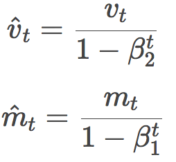
Adam author suggested that β1 is 0.9, β2 is 0.999, and ϵ is 10-8.
In practice, Adam performed very well, converged quickly, and also corrected some of the previous optimization algorithm problems, such as learning rate decay, slow convergence, and loss function oscillation. Generally speaking, Adam is the better choice for adaptive learning rate algorithms.
AMSGrad
At ICLR 2018, Google’s Reddi et al. submitted a paper on the convergence of Adam, pointing out an error in the proof of the convergence of the Adam algorithm. A simple convex optimization problem is constructed as a counterexample to prove that Adam cannot converge on it. In addition, Reddi et al. proposed a variant of the Adam algorithm, AMSGRad, whose main changes are:
Based on the simplicity of the algorithm, Adam's offset correction step is removed.
Only when the current vt is greater than vt-1, vt is applied. In other words, use the larger of the two. This helps to avoid convergence to a sub-optimal solution. The effect of some rare mini-batches that provide large and useful gradients may be greatly weakened by the past mean squared gradient, leading to difficulties in convergence.
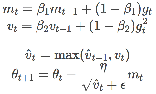
Reddi et al. demonstrated the advantages of AMSGrad over Adam in terms of training loss and test loss on small networks (single-layer MLP on MNIST, small convolutional networks on CIFAR-10). However, some people have conducted experiments on a larger model and found that there is no significant difference between the two (by the way, whether the bias correction of Adam and AMSGrad is turned on has little effect).
Visual optimization algorithm
Let's take a look at two animations below, hoping that they will help intuitively understand the training process of the network.
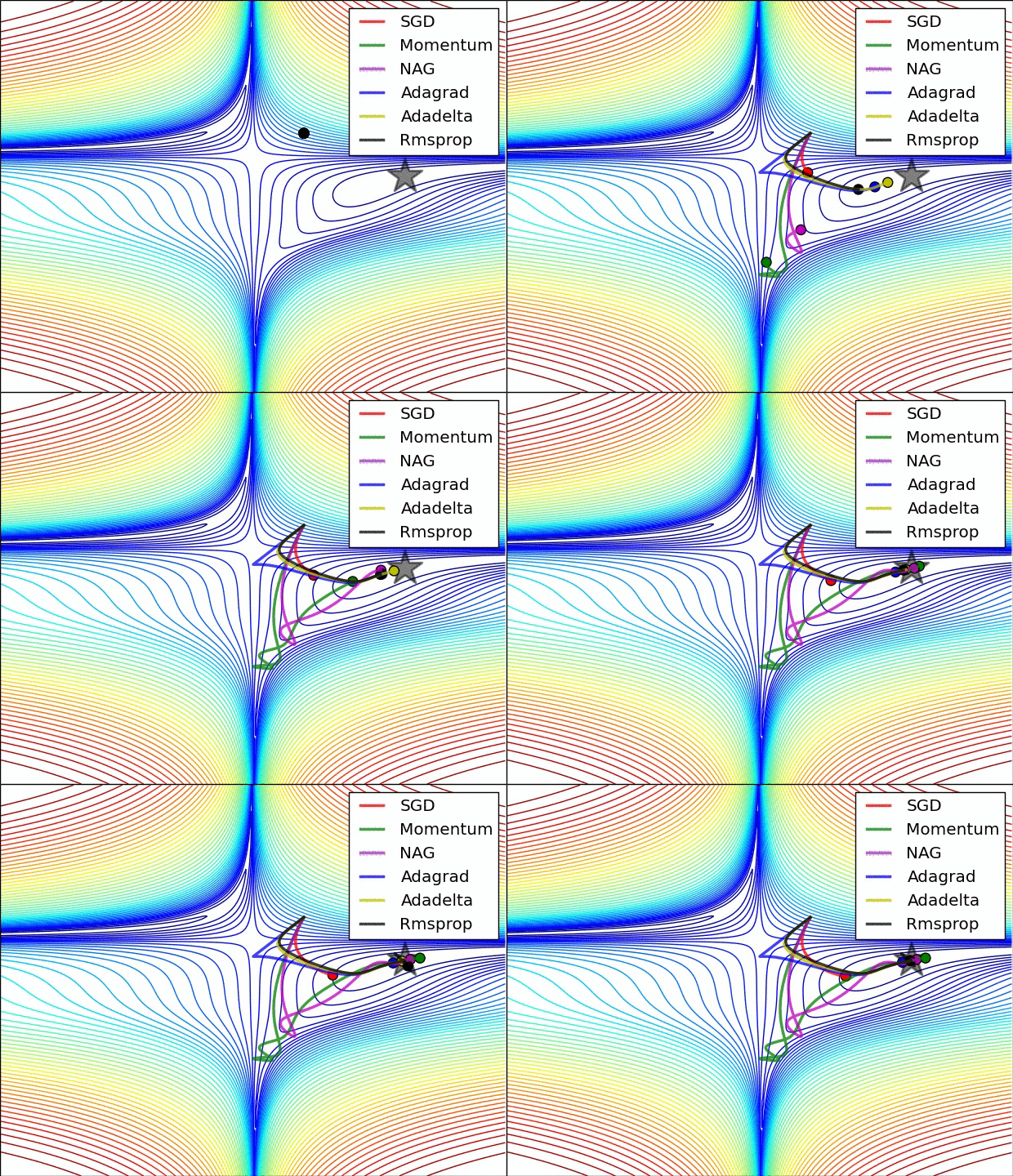
The figure above is the contour map of the error plane. From the figure, we can see that the adaptive learning rate method has completed the convergence cleanly. The convergence of SGD, momentum method, and NAG is very slow. Among them, the momentum method and NAG ran happily in one direction under the action of momentum. In contrast, NAG reacted faster. SGD didn't overshoot, but unfortunately it failed to converge to the optimal value.
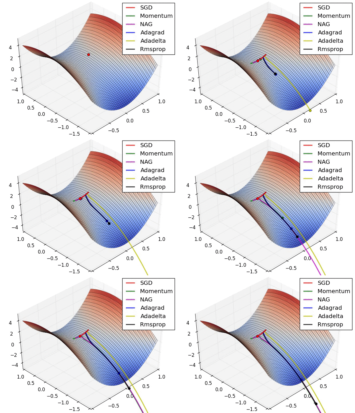
The figure above demonstrates the performance of different optimization algorithms at saddle point. We can see that the adaptive learning rate method got rid of the saddle point without any muddle. Momentum method and NAG finally escaped after hovering at the saddle point for a long time, and SGD finally got stuck in the saddle point and couldn't extricate itself.
The above two animations were produced by Alec Radford.
Which optimization algorithm should be used?
Unfortunately, there is no clear answer to this question. Here are only some suggestions:
Currently, the most commonly used optimization algorithms are SGD, Momentum, RMSProp, AdaDelta, Adam.
On sparse data, it is generally recommended to use an adaptive learning rate algorithm.
On highly complex models, it is recommended to use adaptive learning rate algorithms, which usually converge faster.
In other problems, the use of adaptive learning rate algorithms can usually achieve better performance. At the same time, it also brings an additional benefit: you don't have to worry about setting the learning rate.
In general, Adam is a popular choice among adaptive learning rate algorithms.
Considering the convenience of hyperparameter adjustment, the choice of optimization algorithm also depends on your familiarity with different algorithms.
Adam has better robustness under different hyperparameters, but sometimes you may need to adjust the value of η.
Super Millionaire PCB Board,juegos,casino machines,pcb board
Guangzhou Ruihong Electronic Technology CO.,Ltd , https://www.callegame.com