How to give machines the ability to learn independently has always been a research hotspot in the field of artificial intelligence.
Reinforcement learning and breadth learning
How to give machines the ability to learn independently has always been a research hotspot in the field of artificial intelligence. In more and more complex real-world scene tasks, it is necessary to use deep learning and width learning to automatically learn the abstract representation of large-scale input data, and use this representation as a basis for self-incentive reinforcement learning to optimize problem-solving strategies. The successful application of deep and width reinforcement learning technology in the fields of games, robot control, parameter optimization, machine vision, etc., makes it considered an important way towards general artificial intelligence.
Chen Junlong, a lecturer professor at the University of Macau and vice chairman of the Chinese Society of Automation, gave a report entitled "From Deep Reinforcement Learning to Width Reinforcement Learning: Structure, Algorithms, Opportunities, and Challenges" in the 5th Frontier Workshop on Intelligent Automation Discipline of the Chinese Society of Automation
Professor Chen Junlong's report can be roughly divided into three parts. First, the structure and theory of reinforcement learning are discussed, including Markov decision process, mathematical expressions of reinforcement learning, strategy construction, estimation and prediction of future returns. Then we discussed how to use deep neural network learning to stabilize the learning process and feature extraction, and how to use the width learning structure and reinforcement learning. Finally, the opportunities and challenges brought by deep and wide reinforcement learning are discussed.
Reinforcement learning structure and theory
Professor Chen uses the following diagram to briefly describe the reinforcement learning process. He introduced that the so-called reinforcement learning is that when the agent completes a certain task, it interacts with the environment through action A. Under the action of action A and the environment, the agent will generate a new state, and the environment will give an immediate Return. In this cycle, after several iterations of learning, the agent can finally learn the optimal action to complete the corresponding task.
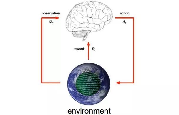
When it comes to reinforcement learning, you have to mention Q-Learning. Then he used another example to introduce the principle of reinforcement learning Q-Learning.
Q-learning
Suppose there are 5 rooms on a floor, and the rooms are connected by a door, as shown in the following figure. The room number is 0 ~ 4, the outside of the floor can be regarded as a large room, number 5.
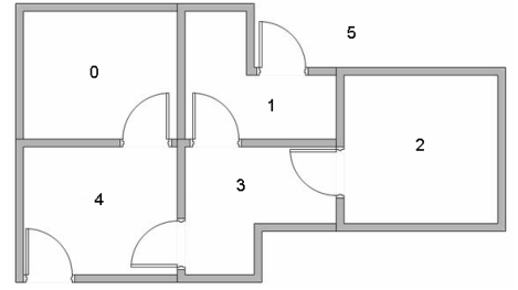
A graph can be used to represent the above-mentioned rooms. Each room is regarded as a node, and each door is regarded as an edge.
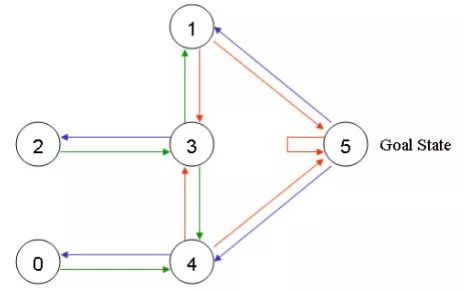
Place an agent in any room and hope it can walk out of the building, which can also be understood as entering room 5. You can use entering room 5 as the final goal, and give the door that can directly reach the target room a reward value of 100, and those that are not connected to the target room are given a reward value of 0. So you can get the following figure.
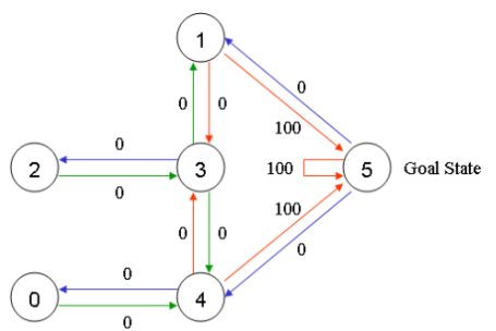
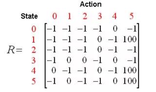
According to the above figure, the reward table can be obtained as follows, where -1 represents a null value, indicating that there is no edge connection between nodes.
Add a similar Q matrix to represent what the agent has learned from experience. The rows of the matrix represent the current state of the agent, and the columns represent the possible actions to reach the next state.
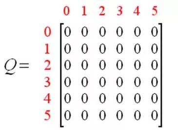
Then Professor Chen introduced the conversion rules of Q-Learning, namely Q (state, action) = R (state, action) + Gamma * Max (Q [next state, all actions]).
According to this formula, the value of an element in matrix Q is equal to the sum of the value of the corresponding element in matrix R and the learning variable Gamma multiplied by the maximum reward value of all possible actions to reach the next state.
In order to understand how Q-Learning works, Professor Chen gave a few examples.
First set Gamma to 0.8, the initial state is room 1.
For state 1, there are two possible actions: reaching state 3, or reaching state 5. Through random selection, choose to reach state 5. What happens when the agent reaches state 5? Looking at the sixth row of the R matrix, there are 3 possible actions to reach state 1, 4 or 5. According to the formula Q (1, 5) = R (1, 5) + 0.8 * Max [Q (5, 1), Q (5, 4), Q (5, 5)] = 100 + 0.8 * 0 = 100, Since the matrix Q is still initialized to 0 at this time, Q (5, 1), Q (5, 4), Q (5, 5) are all 0, so the result of Q (1, 5) is 100, because immediate The reward R (1,5) is equal to 100. The next state 5 now becomes the current state. Since state 5 is the target state, it is counted as completing one attempt. The agent's brain now contains an updated Q matrix.
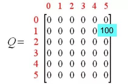
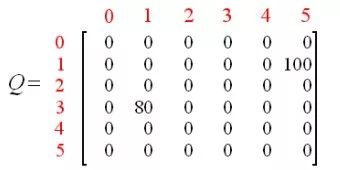
For the next training, state 3 is randomly selected as the initial state. Looking at the fourth row of the R matrix, there are 3 possible actions to reach states 1, 2 and 4. Randomly choose to reach state 1 as the current state action. Now, looking at the second row of the matrix R, there are 2 possible actions: reaching state 3 or state 5. Now calculate the Q value: Q (3, 1) = R (3, 1) + 0.8 * Max [Q (1, 2), Q (1, 5)] = 0 + 0.8 * Max (0, 100) = 80 , Using the matrix Q updated in the previous attempt: Q (1, 3) = 0 and Q (1, 5) = 100. Therefore, the result of the calculation is Q (3,1) = 80. Now, the matrix Q is as follows.
After the agent learns more knowledge through multiple experiences, the value in the Q matrix will reach the convergence state. as follows.
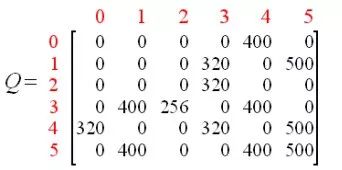
By reducing all non-zero values ​​in Q by a certain percentage, it can be standardized, and the results are as follows.
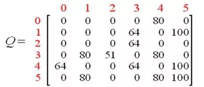
Once the matrix Q is close to the convergence state, we know that the agent has learned the best path to the target state.
So far, Professor Chen has introduced Q-learning briefly. Through the above introduction, we can roughly summarize the six characteristics of reinforcement learning:
Unsupervised, only reward signals
No need to guide learners
Non-stop trial and error
Rewards may be delayed (sacrificing short-term gains in exchange for greater long-term gains)
Need to explore and develop
The interaction between goal-oriented agents and uncertain environments is a global problem
Four elements:
1. Strategy: What to do?
1) Determine the strategy: a = π (s)
2) Random strategy: π (a | s) = p [at = a | st = s], st∈S, at∈A (St), ∑π (a | s) = 1
Second, the reward function: r (while the state transitions, the environment will feedback a reward to the agent)
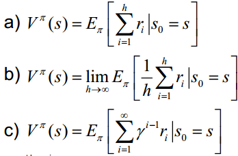
3. Cumulative reward function: V (the quality of a strategy depends on the cumulative reward after long-term execution of this strategy). Common long-term cumulative rewards are as follows:
Fourth, the model: used to represent the environment where the agent is located, is an abstract concept, very useful for action decision-making.
All reinforcement learning tasks are Markov decision-making processes. Professor Chen's introduction to MDP is as follows.
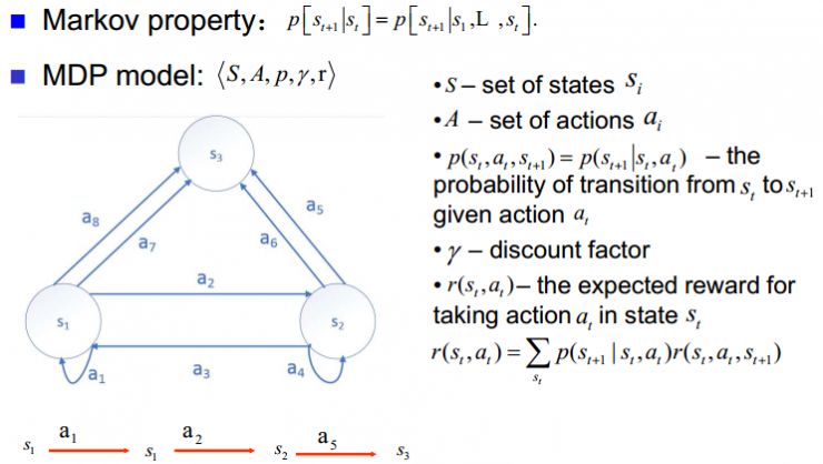
A Markov decision process consists of a quintuple M = (S, A, p, γ, r). Where S is the state set, A is the action set, p is the state transition probability, γ is the discount factor, and r is the reward function.
Professor Chen mentioned the two major challenges facing reinforcement learning at the end of the introduction to reinforcement learning.
Reliability distribution: the previous action will affect the current reward and the global reward
Exploring and pioneering: use existing strategies or develop new strategies
Q-Learning can solve the problem of reliability allocation. The second problem can be solved using ε-greedy algorithm, SoftMax algorithm, Bayes bandit algorithm, UCB algorithm, etc.
Value functions (a prediction of future rewards) can be divided into state value functions and behavior value functions.
1. State value function Vπ (s): starting from the state s, the expected return obtained by taking actions according to the strategy π,
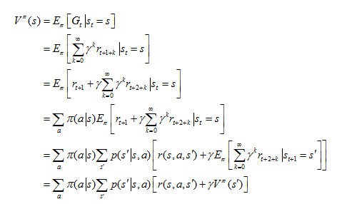
Also known as Bellman equation.
2. Behavioral value function Qπ (s, a): after taking behavior a from state s, and then taking action according to strategy π, the expected return,
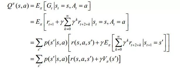
The Bellman equation is also called action-value function.
Similarly, the corresponding optimal value function is given as:
1. The optimal value function V * (s) is the maximum function on all strategies:

2. The optimal behavior value function Q * (s, a) is the maximum behavior value function on all strategies:

Thus to the Bellman optimal equation:

And the corresponding optimal strategy:

Professor Chen introduced the method of solving reinforcement learning, which can be divided into the following two situations:
Method with known model: Method with unknown dynamic programming model: Monte Carlo method, time difference algorithm
Professor Chen further introduced two different methods in the time difference algorithm: the different strategy time difference algorithm Q-learning and the same strategy time difference algorithm Sarsa, the main difference between the two lies in the choice of at + 1,

Ordinary Q-learning is a tabular method, suitable for the case where the state space and the action space are discrete and the dimension is relatively low; when the state space and the action space are high-dimensional continuous or a state that has never occurred, ordinary Q-learning cannot be handled. In order to solve this problem, Professor Chen further introduced the deep reinforcement learning method.
Deep reinforcement learning
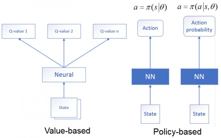
Deep reinforcement learning is a combination of deep neural network and reinforcement learning. It uses the deep neural network to approximate the value function, and uses the method of reinforcement learning to update.
1. Based on the value network: The state is used as the input of the neural network. After the neural network analysis, the value function of all actions that the current state may perform at the time of output is to generate the Q value using the neural network.
2. Based on the strategy network: The state is used as the input of the neural network. After the neural network analysis, the output is the actions that the current state may take (deterministic strategy), or the probability of each action that may be taken (random strategy).
Professor Chen also mentioned the DQN algorithm proposed by Deepmind in Playing Atari with Deep Reinforcement Learning (DRL) in 2013. Deep Q-learning uses the end-to-end fitting Q value of the deep neural network and uses the Q-learning algorithm for the value Update. DQN uses experience playback to train the reinforcement learning process, and sets the target network to handle the TD deviation in the time difference algorithm separately.
Based on the above, Professor Chen further introduced another classic time difference algorithm, the Actor-Critic method, which combines the advantages of value functions (such as Q learning) and policy search algorithms (Policy Gradients), where Actor refers to Strategy search algorithm, Critic refers to Qlearning or other value-based learning methods, because Critic is a value-based learning method, so it can be updated in one step and calculate the reward and punishment value of each step, compared with traditional PolicyGradients Improve the learning efficiency, the strategy structure Actor is mainly used to select actions; and the value function structure Critic is mainly used to evaluate the action of the Actor, the agent selects the action according to the Actor's strategy, and applies the action to the environment, Critic according to the environment The immediate reward is given, the value function is updated according to the immediate reward, and the time difference error TD-error of the value function is calculated at the same time. By feeding back TDerror to the actor, the actor is instructed to update the strategy better, thereby making it better. The selection probability of actions increases, while the selection probability of worse actions decreases.
Width learning
Although deep structured networks are very powerful, most networks are plagued by extremely time-consuming training processes. First, the structure of deep networks is complex and involves a large number of hyperparameters. In addition, this complexity makes the theoretical analysis of deep structures extremely difficult. On the other hand, in order to obtain higher accuracy in the application, the depth model has to continuously increase the number of network layers or adjust the number of parameters. Therefore, in order to improve the training speed, the width learning system provides an alternative method for deep learning networks. At the same time, if the network needs to be expanded, the model can be efficiently reconstructed through incremental learning. Professor Chen also emphasized that in terms of improving accuracy, width learning is to increase nodes rather than increase the number of layers. Based on the efficiency of reinforcement learning, Professor Chen pointed out that width learning and reinforcement learning can be combined to produce width reinforcement learning methods, and it can also be applied to text generation, robotic arm grabbing, and trajectory tracking control.
At the end of the report, Professor Chen mentioned the following points in the future challenges of reinforcement learning:
Safe and effective exploration
Overfitting problem
Multi-task learning problem
Reward function selection
Instability issues
Dock Station Type C,7-Port USB Charging Station Dock,7-Port Charging Station,Type C USB HUB,7 in 1 USB HUB C Docking Station
Shenzhen Konchang Electronic Technology Co.,Ltd , https://www.konchangs.com